Asymptotic behavior

Before reading this article, you must have already read the article about best and worst case in algorithm analysis. If you haven’t read it yet, click here and check it out.

In a simplified and more objective way, the asymptotic behavior can be understood as the growth curve of the function generated by the algorithm analysis process.

It is known that the objective of algorithm analysis is to find a Closed-form expression (function) T(n) that represents the number of instructions executed by the algorithm as a function of its input n.

For example: the algorithm findMax() (in the worst case) has complexity T(n)=4n. This means that if your input n is equal to 4 (an array of size 4), the number of instructions executed by the algorithm will be equal to:

• T(4) = 4*4 = 16 instructions.

Likewise, if the input n is equal to 10 (an array of size 10), the number of instructions executed by the algorithm will be equal to:

• T(10) = 4*10 = 40 instructions.

The functions T(n) found by the analysis process are of great importance to measure the efficiency of the algorithms. Computer science uses these T(n) functions to separate algorithms into specific performance classes. And it does this by analyzing its “asymptotic behavior”.

To begin to understand the concept of asymptotic behavior, we need to graph the function and observe how the number of instructions grows as a function of the value of the input n. To this end, we will analyze the T(n) functions of three hypothetical algorithms in the next section. Are they:

• Algorithm 1. Complexity: T(n)=7
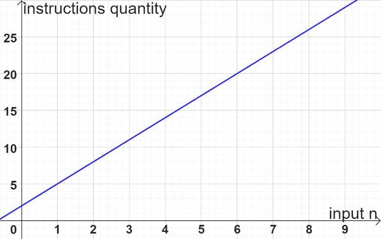
• Algorithm 2. Complexity: T(n)=3n+2
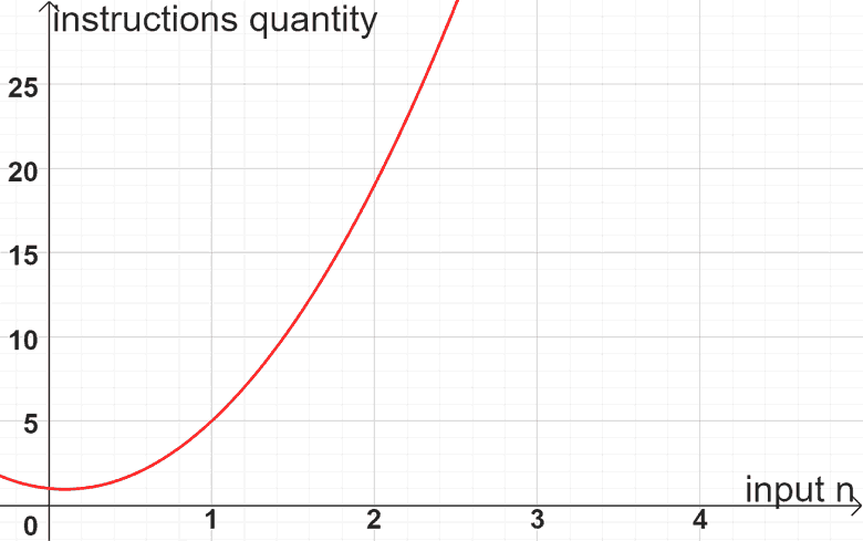
• Algorithm 3. Complexity: T(n)=5n²-n+1

Functions growth curve

For each of the algorithms, we will create a graph: (input size n) x (quantity of instructions executed).

Asymptotic behavior of algorithm 1: T(n)=7

This is a constant complexity algorithm. If we look at the graph of the function illustrated below, we can see how constant its behavior is.

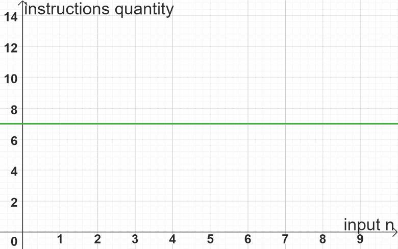
It can be seen in the graph above that the quantity of instructions executed (vertical axis) does not grow as a function of values n (horizontal axis). The number of instructions always remains equal to 7.

Asymptotic behavior of algorithm 2: T(n)=3n+2

This is a linear complexity algorithm. If we look at the graph of the function illustrated below, we can see that the quantity of instructions executed by the algorithm (vertical axis) grows linearly, in relation to the values of n (horizontal axis).

Asymptotic behavior of algorithm 3: T(n)=5n²-n+1

Algorithm 3 has quadratic complexity. If we look at the graph of the function illustrated below, we can see that the quantity of instructions executed by the algorithm (vertical axis) grows quadratically in relation to the values of n (horizontal axis).

Comparison between algorithms

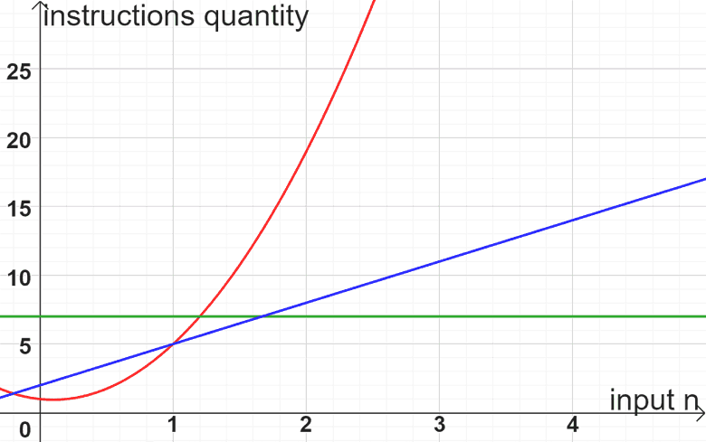
When we superimpose the graphs of the complexity functions of the three algorithms (image below), we can see the growth trend of each of the functions. Notice how the quadratic function tends to present an ever-increasing quantity of instructions for each new size n of the input! This means that the quadratic algorithm is less efficient than the other two, which have a smaller growth trend.

A mistaken asymptotic behavior

Let’s look at a very illustrative example to show the importance of the asymptotic behavior of algorithms. An analysis was performed on two algorithms (A and B) which resulted in the following complexity functions:

Algorithm A

Algorithm B

Question: What is the most efficient algorithm?

See below a table that shows the quantity of instructions executed, by each one of them, for the initial values of n:

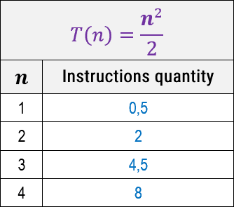
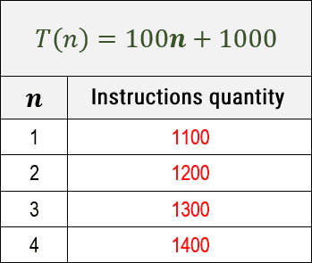
Apparently (looking at the table) we are tempted to say that algorithm A is more efficient because it presents much smaller amounts of instructions for the same values of n.

But observe below what happens when we analyze the quentity of instructions for larger values of n:

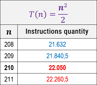
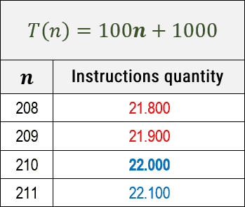
Note that up to a value of n=209, algorithm A is more efficient than B, but from a value of n=210 things change and algorithm B becomes more efficient than A.

The multiplicative and additive constants, respectively 100 and 1000 (in the function of algorithm B), give the false impression that it is less efficient, but they only postpone the inevitable.

See below the graph plotted for both functions. Notice how, starting from the value of n=210, the quantity of instructions executed by algorithm B is surpassed by that of algorithm A:

What we have just done in this example was analyze the asymptotic behavior of the two algorithms. We analyzed the growth trend of algorithm instructions when n has a very large value, when n tends to infinity (n → ∞).

The fact that algorithm A is quadratic already gives us the clue that, for very large values of n (n → ∞), its quantity of instructions will exceed the quantity of instructions of algorithm B, which in turn is linear. For this reason, all additive and multiplicative constants of the complexity function of an algorithm have no impact on its asymptotic behavior (its tendency to grow on the graph).

In this way, it is understood that neither the denominator 2 (of algorithm A) nor the factor 100 and the portion 1000 (of algorithm B) can prevent algorithm B from being more efficient than A for large values of n.

Exercise

So that you can practice the concept of asymptotic behavior of functions, try to solve the proposed exercise.

• Algorithm A: T(n) = n(n+5)
• Algorithm B: T(n) = 10n+10

Graphically analyze the time complexity functions T(n) of algorithms A and B above and determine:

1. What is the “most efficient” and “less efficient” algorithm?
2. At what value of n does the “less efficient” outperform the “most efficient”

Continue your studies in this course and read the next article on “asymptotic classes” in algorithm analysis.